AA 279B · Advanced Space Mechanics
Space Debris &Collision Avoidance
Duncan Eddy · November 10, 2026
Stanford University
Welcome. Today: how a satellite operator actually avoids collisions, end to end, and what you need to be ready to do if you operate a spacecraft. Every figure is generated by a small open-source script you can run yourself (repo link at the end).
The Earth and orbits draw on this click.
Relative speed -- km/s Altitude -- km Crossing angle -- ° Predicted miss distance (public element sets, SGP4) -- m Actual miss distance 0m
Geometry reconstructed from the last public element sets before the event (Space-Track GP history , SGP4) · scripts/debris_clouds.py
Reconstructed with SGP4 from Space-Track GP history: the element sets just before the collision (Iridium epoch 2009-02-09 18:49, Cosmos 11:57, so about a day old). SGP4 predicts a 701 m miss (an independent Vallado sgp4 check gives 698 to 701 m); CelesTrak's SOCRATES listed 584 m. Neither was near the top of anyone's list. Point: a public-catalog miss distance of hundreds of meters is well inside the uncertainty. Note the near-perpendicular crossing; that is typical of LEO conjunctions between different orbital planes, and why relative speeds are so high.
Fragments ever cataloged -- Still in orbit, November 2026 --
Space-Track SATCAT and GP , propagated with SGP4 · scripts/debris_clouds.py
Positions of the surviving fragments right now. The clouds have spread around the whole orbit and the planes have drifted apart due to J2, so the debris threatens a whole altitude shell, not just the original orbits.
Starlink close approach video
deck/img/starlink-near-miss.mp4
Maneuver count: SpaceX semiannual report to the FCC filed 2026-07-01 (Dec 2025 to May 2026), at a Pc threshold of 3e-7 vs the industry-standard 1e-4. Video: @Starlink post, 2026-10-06, arguing that operators maneuvering without sharing their planned trajectory is the biggest risk in LEO.
SpaceX semiannual Starlink report to the FCC, July 2026 · video: @Starlink, October 6, 2026
Sarah Scoles, "Two Satellites Almost Crashed. Here's How They Dodged It," WIRED , February 14, 2019
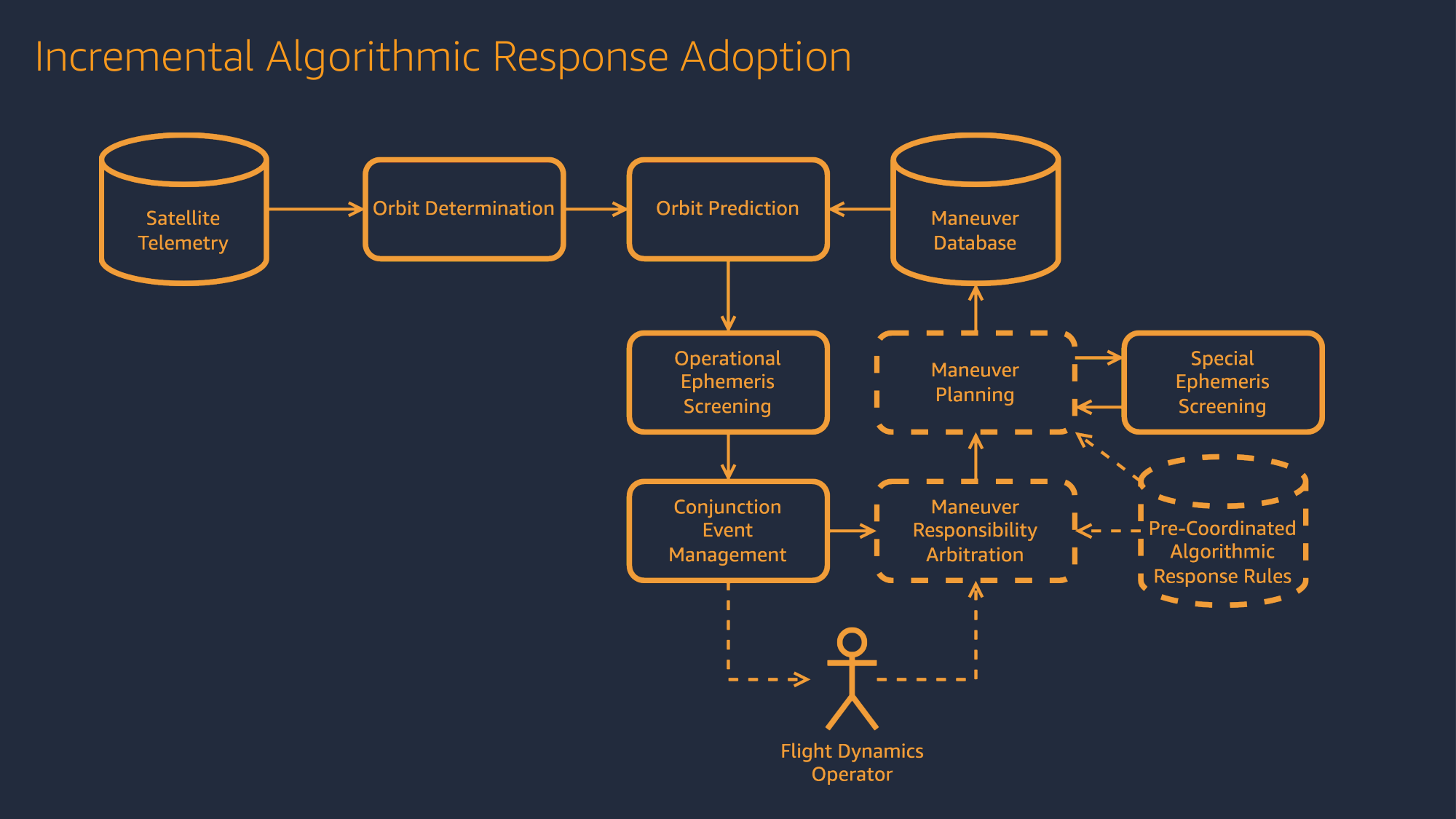
D. Eddy, "Operator CDM Response Coordination," SSA Operators Workshop, June 3, 2022, slide 12
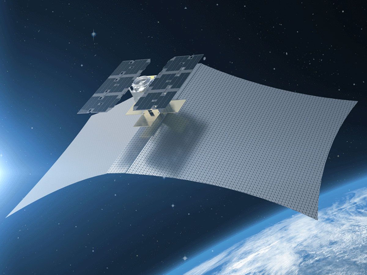
Capella story. A newly launched satellite, thrusters not commissioned yet, so no ability to maneuver. The call came from the Space Defense Squadron doing conjunction assessment (19 SDS since 2022; 18 SDS before). Pause before the next slide. Ask the room what they would do before telling how it resolved. Right: slide 12 of the first public talk on Project Kuiper's conjunction response practices (2022). Solid boxes are the automated pipeline (telemetry, OD, prediction, operational ephemeris screening, conjunction event management); dashed boxes were adopted incrementally (maneuver responsibility arbitration, maneuver planning, pre-coordinated response rules) with the flight dynamics operator in the loop.
How do you avoid a crash when you drive?
Expected: look around, mirrors, sensors, brake or steer. Everything is local: what you see right now is what you need.
Highway speed: -- mph-- mph).
You can see at least -- ft
Hard braking at -- g, after a -- s reaction time.
You stop in -- ft
In orbit
Orbion Aurora datasheet (2021) ; K2 Space · scripts/avoidance_budget.py
Slow approaches do exist (right after deployment, rendezvous), but they are rare and low energy. Space-based tracking from many satellites (e.g. SpaceX's Stargaze) helps, but only works at enormous scale. Displacement is 0.5 a t² over the 8.5 s warning, thrusting the entire time (best case: no slew, no spin-up). Orbion Aurora: 19 mN at 300 W, on a 100 kg smallsat (the datasheet lists spacecraft of 70 kg and up). K2 Space: 1 N on a 2,000 kg bus. Even an idealized instantaneous 1 m/s impulse would move you only 8.5 m (checked with brahe two-body propagation). Compare with a typical combined hard-body radius of 10 to 20 m and position uncertainties of hundreds of meters.
Median closing speed of this week's close approaches: -- mph-- km/s).
A sensor that sees 100 km ahead gives you -- s
Thrust the whole time: Orbion Aurora (19 mN, 100 kg sat) or K2 Space (1 N, 2,000 kg bus).
550 km circular orbit: a = -- km, v = -- km/s, period -- min. Burn along the velocity one orbit before closest approach.
Orbion Aurora, 100 kg 1 N, 2,000 kg K2 bus
Δv from 8.5 s of thrust \(\Delta v = (F / m)\, t\) -- --
Same thrusters and the same burn duration as the previous slide, but performed one orbit (about 96 min) before the encounter instead of in the last seconds.
Change in semi-major axis \(\Delta a = 2a\,\Delta v / v\) -- --
A tangential Δv on a circular orbit changes the energy, so the semi-major axis: Δa = 2aΔv/v.
Change in orbital period \(\Delta T = 3\pi\,\Delta a / v\) -- --
T ∝ a^(3/2), so ΔT/T = (3/2)Δa/a, which is ΔT = 3πΔa/v for a circular orbit. Milliseconds.
Along-track shift one orbit later \(\Delta s \approx v\,\Delta T = 3\pi\,\Delta a\) -- --
Same burn in the last 8.5 s \(\Delta s = \tfrac{1}{2}(F / m)\, t^2\) -- --
scripts/avoidance_budget.py
One orbit later the satellite arrives a few milliseconds late, which at 7.6 km/s is tens of meters along-track: about 4,000 times more than the same burn spent pushing sideways in the last seconds. The prograde burn raises the orbit, so the satellite lags behind where it would have been.
Early maneuvers work by changing the orbital period, not by pushing the satellite aside. The along-track offset grows by about 3πΔa every orbit.
This is why lead time matters so much in the maneuver trade space later: the same Δv buys more separation the earlier it is applied.
Avoiding a collision in space requires advance warning, which requires tracking objects in orbit and predicting close approaches before they happen.
This is the key difference with terrestrial collision avoidance. The problem is global and predictive, not local and reactive.
Sensing from orbit can help, but only at enormous scale: SpaceX's Stargaze uses the star trackers on thousands of Starlink satellites.
Stargaze: SpaceX's SSA system using Starlink star trackers, opened to outside operators in August 2026. It does not see small debris and does not replace ground radar.
Share Where are you going?
Roadmap. The same four questions for each stage. Decide is the real challenge: everything before it feeds a decision under uncertainty. This graphic returns at each section start with the current section in red.
Space-Track GP catalog · scripts/catalog.py
Click a category on the right to turn it off or on. Every dot is a real cataloged object at one instant. Only objects large enough to track (roughly 10 cm in LEO, about 1 m in GEO) are here; models estimate on the order of a million objects larger than 1 cm.
How do we know where objects in space are?
Let the room answer: radar, telescopes, GPS on the satellite itself. Then each measurement type.
GPS position (and velocity)
Radar azimuth, elevation,
Telescope azimuth, elevation,
Each sensor has a measurement model h(x). Bottom row: two-way ranging through the operator's own TT&C link, satellite laser ranging (SLR) for retroreflector-equipped satellites, and Doppler range-rate from the carrier (e.g. DORIS, or the TT&C downlink). Initial orbit determination (Gauss, Gibbs, Lambert-based) gets a first state from a few observations; a batch least-squares or a sequential filter (EKF/UKF) refines state and covariance; then you propagate.
From measurements to an orbit: initial orbit determination (Gauss, Gibbs, Lambert-based) gives a first state; batch least squares or a sequential filter (EKF/UKF) refines the state and covariance; then you predict.
-- , 24 hours: -- radar passes-- h
Between passes the catalog only has predictions. That is where uncertainty grows, and why "ephemeris age" matters later. Visibility here is purely geometric; telescopes also need darkness and a sunlit target, so only radar passes are counted. This is the textbook (Vallado) sensor list, not the full current network; six sites have no published limits and use open defaults.
Eglin radar (brahe SSN dataset) · scripts/rideshare_tracks.py
A rideshare dispenser at 525 km releases 20 satellites a minute apart, each with 0.5 to 1.5 m/s separation velocity. Eglin radar measurements (azimuth, elevation, range; 0.02 deg and 30 m noise) every 2 s on two passes, shown as a sky plot: zenith at the center, horizon at the edge, the faint red ring is the 10 deg elevation mask. The radar gets points, not names. Click: the true identity of each point. A few hours after deployment they arrive within about 20 s of each other; a day later the train has stretched to about 80 s and the order has changed. Every point has to be associated with an object before an orbit can be estimated.
What do we do with all these tracks?
Associate them with objects, estimate each object's orbit, and keep those orbits up to date in a catalog.
Let the room answer first. Track-to-object association (multi-hypothesis tracking), orbit determination, and catalog maintenance.
Let the room answer first.
A maintained list of tracked objects and their current orbits. Several exist, each with a different set of objects.
Space-Track.org
Run by the US Space Force's 18th Space Defense Squadron, whose mission is to maintain the satellite catalog.
When people say "the catalog", they almost always mean this one.
CelesTrak
Public and free. Redistributes the Space-Track data and adds supplemental orbits from operators' own ephemerides.
TraCSS, space-safety.com
Operator coordination platforms (Office of Space Commerce; SpaceX) with their own catalogs. Not public.
space-track.org · celestrak.org · TraCSS · space-safety.com
Catalog maintenance: associate each new track with a known object or declare a new one (launches, breakups, deployed parts, satellites releasing others). 18 SDS (Vandenberg) maintains the US catalog; conjunction assessment for operators moved to 19 SDS in 2022. CelesTrak (T.S. Kelso) redistributes GP data and publishes supplemental GP derived from operator ephemerides (e.g. Starlink). TraCSS (Office of Space Commerce, pilot) and SpaceX's space-safety.com screen operator-shared ephemerides; neither is a public catalog.
Generate hypotheses. The new track could belong to any object it plausibly matches (gating), be a new object, or be a false alarm. Score them. How well the track fits each object's predicted orbit, given its uncertainty, plus prior rates of new objects and false alarms. Extend. When the next track arrives, branch every surviving hypothesis again. Prune and commit. Drop unlikely branches. Commit to an association only once one hypothesis clearly wins.
Track-to-object association is combinatorial: every new track could match several objects. MHT keeps a tree of association hypotheses, scores each with the measurement likelihood against each object's predicted state and covariance plus priors for new objects and false alarms, and prunes as data arrive (N-scan, keep the K best). Leftover tracks that match nothing become uncorrelated tracks (UCTs); objects that stop matching become lost objects.
Developed for NORAD in the 1960s, when numerically integrating the whole catalog was too expensive: mean elements fitted for the semi-analytic SGP4 propagator, which includes a drag term.
Mean elements from Brouwer-Lyddane-style theory plus a drag term (B*). The element set is the result of a fit that only means something together with SGP4.
Mean elements as osculating TLE elements are SGP4 mean elements. Converting them straight to a position and velocity gives the wrong orbit.
TEME used as GCRF SGP4 outputs TEME, not a standard inertial frame. Convert it.
A different propagator Only valid with SGP4. Even from the correct osculating state, a similar numerical propagator drifts away.
scripts/tle_gotchas.py
Click a box to reveal that mistake and its curve, or advance to reveal them in order. ISS, current element set, errors relative to SGP4 in GCRF, log scale. Mean elements as osculating: semi-major axis off by 6.5 km, 12 km error at epoch, 932 km after one day, almost all along-track. TEME vs GCRF: a 0.375° rotation (mostly precession since J2000), so 34 to 45 km of position error from day one. Different propagator: start from SGP4's own state at epoch (the proper mean-to-osculating conversion, SGP4's short-period terms applied) and integrate with J2 to J4 zonals and Harris-Priester drag with Cd·A/m from B*: about 2 km after one day and growing. Small next to the other two, but a TLE is a fit for SGP4, so any other propagator adds its own error on top of SGP4's own km-level error.
Let the room look at the field layout. The catalog number field is five characters wide (columns 3 to 7), which leads into the next slide.
The catalog ran out of five-digit numbers
On July 11, 2026 the catalog passed 69,999 and jumped to 100000 . Four months later, --
Object 100000 is SARAMAGO (2026-067CY). 70000s: pre-launch/nominal elements, 80000s: analyst objects, 90000s: uncorrelated tracks. Space-Track's legacy TLE output uses Alpha-5 for 100000 to 339999; CelesTrak does not publish TLEs for these. OMM via the Space-Track gp class supports 9-digit IDs.
Many people still call these TLEs.
Space-Track gp class; CelesTrak GP queries with FORMAT=json. Same mean elements, same SGP4, no five-digit limit. brahe reads GP/OMM records directly. The record shown is the same ISS element set as the TLE on the earlier slide, as returned by the Space-Track gp class in JSON. Highlighted: NORAD_CAT_ID (no five-digit limit), REF_FRAME TEME and MEAN_ELEMENT_THEORY SGP4.
Which of ~-- catalog objects pose a risk?
Expected: propagate everything, check distances. Then: how expensive is that?
Hoots, Crawford & Roehrich 1984 · scripts/screening.py
Apsis: altitude ranges must overlap. Path: the orbits must come close somewhere (minimum orbit intersection distance). Phase: both objects must be near that point at the same time. Each is conservative: it can keep pairs that won't conjunct but never drops a real one. Vedant (in the room?) showed object-specific uncertainty-aware apsis thresholds remove 71% of all-vs-all pairs. Here: ISS vs 32,877 objects, 7 days in 30-min windows (11.0M object-windows). Apsis keeps 29%, path 19%, phase 0.2%; fine SGP4 screening of the 25k survivors finds 7 candidate events, and a brute-force run confirms none were missed (7/7, and 316/316 approaches within 35 km). Per object the funnel looks weak (13.5k, 10.8k, 7.3k objects pass in some window): over a week, nodal drift means most orbits at ISS altitude intersect somewhere. These are SGP4 screening hits, not risk.
Why is the screening volume a box that is thin radially and long along-track?
Hint: think back to the GPS vs catalog plot.
Along-track uncertainty grows fastest, so the volume is stretched along the velocity direction. The box rides with the primary; anything that enters it during the screening span is a close approach and goes on to risk assessment.
It will pass -- m-- km/s.
How would you estimate the probability that they collide?
--
Expected: sample from the uncertainty, count hits. Good. How many samples?
CALIPSO vs. Cosmos 2251 debris (NASA CARA test case) · scripts/pc.py
Each sample draws both objects' states from their estimates and covariances, propagates them to closest approach (here: straight-line relative motion near TCA, the same assumption as 2D Pc), and counts a hit when the miss distance is inside the combined hard-body radius. Pc is hits over samples. Click: the running estimate for this conjunction as samples accumulate, with its 95% interval, converging on the Foster value (dashed). After 1,000 samples there is one hit; it takes millions of samples to pin Pc down to a few percent.
Interactive: drag the slider to set the true Pc, click a confidence level and a target relative error. Relative standard error of a binomial estimate: sqrt((1-p)/(N p)). For 10% error at 95% confidence, N ~ 384 (1-p)/p. Each sample needs two high-fidelity propagations to TCA.
1. Assume motion during the encounter is a straight line At -- km/s and -- °, the encounter lasts under a second; covariances stay fixed.
2. Add the two covariances \(C = C_1 + C_2\) is the uncertainty in the position of one object relative to the other.
3. Project onto the encounter plane Only directions perpendicular to the relative velocity matter: -- (1σ).
4. Integrate over the hard-body disk Relative position \(\mathbf{x}\) = primary − secondary is Gaussian around the predicted miss \(\boldsymbol{\mu}\). \(P_c\) is the chance it lands within \(R = R_1 + R_2 =\) -- m of the secondary:
\(P_c = \displaystyle\iint_{\lVert \mathbf{x} \rVert \le R} \mathcal{N}\!\left(\mathbf{x};\ \boldsymbol{\mu},\ C_{2D}\right) dA\)
\(P_c =\) -- (1 in -- ) Monte Carlo with -- samples: -- . Matches NASA CARA on -- test cases (max relative error -- ).
Foster & Estes 1992, NASA JSC-25898; NASA CARA Pc2D_Foster · scripts/pc.py
Fast encounters (LEO, tens of seconds or less in the uncertainty region) make the straight-line, constant-covariance assumptions good. The integral is over the Gaussian of the relative position in the encounter plane, centered on the predicted miss, evaluated over a disk of the combined radius centered on the secondary. Slow encounters (GEO, formation flying) break the assumptions; that is where 3D Pc or Monte Carlo is used.
2D \(P_c\) Foster 1992, Chan, Alfano
Fast encounters, straight-line motion. The workhorse.
3D \(P_c\) Hall et al. (NASA CARA)
Curved relative motion and changing covariance. Slow or long encounters, GEO.
Monte Carlo Sampling from TCA or from epoch
The reference. Use it to check the others when assumptions are in doubt.
NASA CARA Analysis Tools
CARA's tools pick the method based on encounter duration and covariance conditions.
NASA CARA plans a mitigation when \(P_c\) ≥ 1 in 10,000 (10⁻⁴) .
Space Force "emergency" events in LEO: within 3 days, miss < 1 km and \(P_c\) ≥ 1 in 10,000 (10⁻⁴) .
Thresholds are set by policy and differ between organizations.
Spaceflight Safety Handbook v1.7: near-Earth emergency reportable = TCA within 3 days, miss distance at most 1 km and Pc at least 1e-4 (deep space: within 3 days and miss within 5 km). CDMs are posted on Space-Track for Pc at least 1e-7. SpaceX maneuvers at 3e-7.
scripts/covariance_banana.py
Drag uncertainty spreads samples along the curved orbit. In Cartesian coordinates the cloud bends; a Gaussian ellipse no longer describes it and standard Kalman updates and 2D Pc assumptions degrade. Fixes: curvilinear/element coordinates, Gaussian mixtures, particle methods. Drag the slider. Setup: 400 km ISS-like orbit, 500 samples, 20% Cd uncertainty, NRLMSISE-00 drag. At 7 days the along-track spread is 482 km (1σ; MC and linear agree on that), but the Monte Carlo radial spread is 25 km vs 0.8 km linear, with a 17 km mean radial offset: the cloud follows the curved orbit. Same scale on both axes.
STARLINK-4133: the operator's GPS-based ephemeris vs the public catalog element set (GP / TLE)
scripts/starlink_vs_gp.py
STARLINK-4133. The public catalog (GP / TLE) is a radar-and-telescope fit with a simplified propagator; the operator's ephemeris is GPS-based orbit determination with a high-fidelity force model. At the start they differ by about 1 km (GP 8 h old) vs about 1 m operator uncertainty. Along-track dominates: 12 km at 1 day, 77 km at 3 days; radial and cross-track stay under 0.5 km. Remember this for the screening volume. This satellite was picked because its 3-day ephemeris has no planned maneuvers; across 80 random Starlinks the median along-track difference is 24 km at 1 day and 138 km at 3 days, mostly because the GP knows nothing about planned maneuvers (callback to the Starlink post). Note: the operator covariance after ~16 h looks like fixed published values, not propagated uncertainty.
Error source: 35% error in the drag model
scripts/gps_od.py
Truth: 20x20 gravity, NRLMSISE-00 drag, SRP, Sun and Moon. Filter: 20x20 with Harris-Priester drag and a low Cd, so its drag is about 35% too weak (near solar maximum). 6 h of 5 m GPS fixes: about 1 m RMS. Then predict: 4 km along-track at 1 day, 14 km at 2 days, 49 km at 4 days. Along-track grows quadratically: drag error changes semi-major axis, which changes mean motion. Notice the filter's own 3σ (dashed): process noise grows like t^1.5 but a drag bias grows like t², so late in the prediction the covariance stops being honest (covariance realism, later). A real operator would estimate Cd and do better.
Effect of miss distance and uncertainty Keep the miss direction, the covariance shape and the hard-body radius. Set the miss distance (5 m, 197 m, 2 km), scale every 1σ by the same factor, and recompute \(P_c\).
Large σ: the miss distance barely matters At σ = 10 km, misses of 5 m, 197 m and 2 km all give \(P_c \approx 10^{-5}\).
Small σ: \(P_c\) goes to 1 or 0 At σ = 10 m, the 5 m miss (inside R = 15 m) gives 0.8. The 197 m and 2 km misses give less than \(10^{-100}\).
scripts/pc_evolution.py · Alfano 2005 (dilution)
Pc dilution. At the real CDM covariance (σ major 565 m) the 197 m miss gives 1.76e-3. Scale the covariance up and every curve falls together: Pc is small because we do not know, not because it is safe. Scale it down and the curves separate: the 5 m pass (inside the 14.8 m hard-body radius) goes to 1, the 197 m and 2 km passes go to 0. Better ephemerides (operator GPS solutions, SP instead of GP, shared maneuver plans) move you left on this plot. Construction: the CDM's combined encounter-plane covariance and hard-body radius are kept; only the predicted miss distance is replaced (5 m, 197 m, 2 km, same direction) and the covariance is multiplied by k^2. Pc is the Foster 2D integral, not an Alfano formula; Alfano 2005 is the reference for the dilution effect.
Drag the miss distance to add a fourth curve; drag the 1σ slider to move the dot along it. Same CDM covariance shape and hard-body radius as the three fixed curves; Pc is computed in the browser with the same Foster integral.
Public catalog GP / TLE mean elements for SGP4, on Space-Track for anyone with an account.
STARLINK-4133: about 1 km off at the start, 77 km along-track after 3 days. No covariance.
SP catalog Special Perturbations ephemerides and state vectors from the 18 SDS High Accuracy Catalog , refit every 8 h.
Requires an SSA Sharing Agreement (Advanced CA). No covariance in the files.
Operator ephemerides Each operator's own orbit determination, often GPS, with planned maneuvers.
Shared on Space-Track and space-safety.com, usually with covariance.
With SP ephemerides an operator can screen its own trajectories on demand. \(P_c\) still needs a covariance for the other object.
USSF Spaceflight Safety Handbook for Satellite Operators v1.7, pp. 3–8
Public GP/TLE: SGP4 mean elements, basic level, any registered Space-Track user. SP: 18 SDS runs Special Perturbations OD several times a day and updates the High Accuracy Catalog (HAC); the catalog is refit and propagated 7 days (near-Earth) or 10 days (deep space) every 8 hours. Advanced CA (SSA Sharing Agreement, requested through the Orbital Data Request process) adds access to propagated SP ephemeris and SP state vectors for the unclassified catalog, both without covariance. Operator ephemerides: OEM or Modified ITC on Space-Track, screened by 19 SDS; SpaceX space-safety.com. This is what lets an operator run its own screening, for example with brahe, instead of waiting hours for 19 SDS results. Covariance for the secondary comes from CDMs or your own estimate.
Hands up
\(P_c = 10^{-3}\), three days before closest approach. Do you maneuver?
Now · Wait for the next update · No
Take a count for each option. There is no single right answer, which is the point.
scripts/pc_evolution.py
Simulation: covariance growth fitted to real data (Starlink operator ephemerides for the primary, 53 NASA CARA test CDMs for the secondary), estimate errors drawn from each update's covariance. Of truly safe 500 m passes, 38% crossed 1 in 10,000 at some update a day or more out; none were still above it at 6 h. Of true 50 m threats, 99% are above it at 6 h. Early on, you can't tell which is which. Dilution: for this geometry Pc peaks (2e-3) when the covariance is about 0.74 times its CDM size; more uncertainty can make Pc go down, which does not mean safer. Caveat: real CDM updates are correlated; these draws are independent.
Updates? Will we get more measurement updates before TCA?
How will dynamics uncertainty change \(P_c\) by then?
Data? Will the other operator share their ephemeris?
Is it built correctly: frame, covariance, planned maneuvers?
Their action? Can they maneuver: thrusters or differential drag?
Will they? When, and in which direction?
Net effect? What does each of these do to the risk?
Up or down, and by how much?
Smaller: our own thruster performance, the other object's size and attitude.
Maneuvering costs fuel and interrupts the mission. Waiting buys information but makes the maneuver more expensive and riskier.
Industry standard: fixed rules (e.g. Pc above 1e-4 at T-24h, maneuver). Better: trade-space tables of maneuver size vs time vs residual risk. Really: a POMDP. Grace Kim's work in SISL: Kim, Eddy, Kochenderfer, "Chance-Constrained Belief-Space Maneuver Planning for Autonomous Collision Avoidance Under Uncertainty," AMOS 2026 (arXiv:2609.13428): in 96 scenarios the planner reached TCA without maneuvering in about 40% of episodes with no terminal-risk violations. Kim, Al-Husseini, Eddy, Kochenderfer, "Semi-Decentralized Multi-Spacecraft Collision Avoidance under Communication Constraints," AAS/AIAA ASC 2026 (arXiv:2607.26570): 28.5% fewer synchronization events than continuous coordination.
All HAC (High Accuracy Catalog) Every object in the SP catalog against every other: near-Earth (period ≤ 225 min) propagated 7 days, deep space 10 days.
Concern list Re-screens the pairs that All HAC flagged, with TCA ≤ 5 days: \(P_c\) ≥ 10⁻⁷ near-Earth, miss ≤ 5 km deep space.
O/O ephemeris vs HAC Your uploaded ephemeris against the SP catalog. Operational files: results 8–12 h after the slot. Special (maneuver) files: as soon as possible, results within 4 h.
O/O vs O/O Operational ephemerides against each other, re-screened every 8 h until less than 8 h (near-Earth) or 12 h (deep space) of the file remains.
USSF Spaceflight Safety Handbook for Satellite Operators v1.7, pp. 5–9 · schedule in EST (EDT is one hour earlier)
19 SDS screens everything at least every 24 h. The catalog is updated and propagated every 8 h (7 days near-Earth, 10 days deep space). One full HAC vs HAC per regime per day, then two concern-list screenings 8 h apart. O/O ephemeris vs HAC: an operational file is screened once, within 8 h of upload; special files are screened as soon as possible and are not screened against other O/O ephemerides. O/O vs O/O: operational files are kept and re-screened every 8 h until less than 8 h (near-Earth) or 12 h (deep space) of ephemeris remains. This is the baseline. If you need faster turnaround, you screen yourself (next slide).
Baseline loop: get a CDM, plan candidate maneuvers, submit them to Space-Track as special ephemerides for screening, wait for results (special files within about 4 h, operational 8 to 12 h), decide which to fly, publish the OEM with the burn on Space-Track so others can plan around you, wait for CDMs on the new OEM, and repeat until TCA. Format: CCSDS OEM (optionally with covariance) or Modified ITC, in MEME J2000. SpaceX's space-safety.com returns screening in under a minute. In-house (step 1): with an SSA Sharing Agreement you can pull SP ephemerides for the whole unclassified catalog and screen candidate maneuvers yourself, on demand, in minutes. The SP files have no covariance, so Pc needs your own estimate for the other object or the CDM values. You still publish the chosen ephemeris so 19 SDS and other operators screen against it.
You launch next year. What do you need to be able to do ?
Collect answers, map them onto the next slide.
Automate flight dynamics Download measurements and determine and predict orbits, automatically
Check that predictions are self-consistent
Share it Publish predicted ephemerides (OEM) and maneuver plans
Have a conjunction response plan Fixed rules, trade-space tools, or a solved decision policy
On call at any hour
Have the process before launch. The first warning can arrive before your thrusters are commissioned.
Callback to the Capella story.
All free. The CARA handbook is the best single read on the whole lifecycle.
Doing this requires time systems, reference frames, propagation, estimation, data formats and catalog clients.
Does every new operator have to build all of this?
Commercial tools (STK, FreeFlyer) are expensive with dated interfaces. Open-source packages are narrow in scope or not validated. Frames and time are where subtle bugs live.
Time & frames time · eop · frames · coordinates · spice · attitude
Dynamics orbits · orbit_dynamics · propagators · integrators · relative_motion
Analysis events · access · estimation
Data formats ccsds (OEM · OPM · OMM · OCM) · itc · sp3
Clients spacetrack · celestrak · starlink · igs
Tools constants · math · plots · cli
Coming conjunction screening · \(P_c\)
Rust core, Python API, MIT licensed, developed since 2014. Every figure today is a short uv run script built on it.
Rust core, Python API. MIT licensed, developed since 2014. Every major submodule is listed; screening and Pc are in progress.
import brahe as bh
epoch = bh.Epoch (2026 , 11 , 10 , 0 , 0 , 0.0 , time_system=bh.TimeSystem.UTC)
x0 = bh.state_koe_to_eci ([bh.R_EARTH + 525e3 , 0.001 , 97.5 , 30 , 0 , 0 ],
bh.AngleFormat.DEGREES)
force = bh.ForceModelConfig (
gravity=bh.GravityConfiguration.spherical_harmonic (degree=20 , order=20 ),
drag=bh.DragConfiguration (bh.AtmosphericModel.HARRIS_PRIESTER,
area=bh.ParameterSource.value (1.2 ), cd=bh.ParameterSource.value (2.2 )),
third_body=[bh.ThirdBody.SUN, bh.ThirdBody.MOON],
mass=bh.ParameterSource.value (100.0 ),
)
prop = bh.NumericalOrbitPropagator (epoch, x0,
bh.NumericalPropagationConfig.default (), force)
prop.propagate_to (epoch + 3 * 86400.0 )LEO with 20x20 EGM2008 gravity, Harris-Priester drag (1.2 m² area, Cd 2.2), Sun and Moon third-body, 100 kg; propagate 3 days. Runs as shown: pocs/brahe_snippets.py (523 km after 3 days).
bh.load_spice_kernel ("de440s" )
t0 = bh.Epoch (2028 , 12 , 10 , 0 , 0 , 0.0 , time_system=bh.TimeSystem.TDB)
x0 = bh.spk_state (bh.NAIFId.EARTH, bh.NAIFId.SUN, t0) # on Earth's orbit
sun = bh.CentralBody.from_naif_id (bh.NAIFId.SUN)
force = bh.ForceModelConfig.for_body (sun,
gravity=bh.GravityConfiguration.point_mass (),
third_body=[bh.ThirdBody.JUPITER, bh.ThirdBody.VENUS])
def tmi (epoch, x): # trans-Mars injection: 3.2 km/s prograde
x = x.copy ()
x[3 :] += 3200.0 * x[3 :] / np.linalg.norm (x[3 :])
return x, bh.EventAction.CONTINUE
cruise = bh.NumericalOrbitPropagator (t0, x0,
bh.NumericalPropagationConfig.default (), force)
cruise.add_event_detector (
bh.TimeEvent (t0 + 86400.0 , "TMI" ).with_callback (tmi))
cruise.propagate_to (t0 + 204 * 86400.0 ) # passes Mars
Sun-centered propagation (central body from NAIF ID 10, the Sun) with Jupiter and Venus perturbations, starting on Earth's orbit from the DE440s ephemeris. A TimeEvent callback applies a 3.2 km/s prograde burn one day in. Departure date and burn size come from a scan of the 2028-29 window (scripts/mars_transfer.py); the spacecraft passes about 0.46 million km from Mars on day 204. The animation replays the daily states. The snippet runs as shown: pocs/brahe_snippets.py.
Summary
Spacecraft collision avoidance is managed through the intersection of multiple complex systems, all of which are facing strain under increased operational activity.
Repo link with all scripts and the deck, and brahe.space. Questions.